Gapminder#
import japanize_matplotlib
import matplotlib.pyplot as plt
import numpy as np
import pandas as pd
import py4macro
from gapminder import gapminder

# 警告メッセージを非表示
import warnings
warnings.filterwarnings("ignore")
/Library/Frameworks/Python.framework/Versions/3.12/lib/python3.12/site-packages/gapminder/data.py:1: UserWarning: pkg_resources is deprecated as an API. See https://setuptools.pypa.io/en/latest/pkg_resources.html. The pkg_resources package is slated for removal as early as 2025-11-30. Refrain from using this package or pin to Setuptools<81.
  import pkg_resources
Gapminderとは世界規模で見た経済格差をデータで探る有名なサイトであり、一見の価値があるサイトである。そのサイトで使われているデータを整理してパッケージにまとめたのがgapminderである。
Note
MacではTerminal、WindowsではGit Bashを使い、次のコマンドでgapminderをインストールできる。
pip install gapminder
ここではgapminderに含まれるデータを使いpandasのgroupbyというDataFrameのメソッドの使い方の例を紹介する。両方ともデータをグループ化して扱う場合に非常に重宝するので、覚えておいて損はしないだろう。
データ#
<列ラベル>
country:国名continent:大陸year:年lifeExp:平均寿命pop:人口gdpPercap:一人当たりGDP(国内総生産)
データの読み込みと最初の5行の表示
df = gapminder
df.head()
| country | continent | year | lifeExp | pop | gdpPercap | |
|---|---|---|---|---|---|---|
| 0 | Afghanistan | Asia | 1952 | 28.801 | 8425333 | 779.445314 |
| 1 | Afghanistan | Asia | 1957 | 30.332 | 9240934 | 820.853030 |
| 2 | Afghanistan | Asia | 1962 | 31.997 | 10267083 | 853.100710 |
| 3 | Afghanistan | Asia | 1967 | 34.020 | 11537966 | 836.197138 |
| 4 | Afghanistan | Asia | 1972 | 36.088 | 13079460 | 739.981106 |
最後の5行の表示
df.tail()
| country | continent | year | lifeExp | pop | gdpPercap | |
|---|---|---|---|---|---|---|
| 1699 | Zimbabwe | Africa | 1987 | 62.351 | 9216418 | 706.157306 |
| 1700 | Zimbabwe | Africa | 1992 | 60.377 | 10704340 | 693.420786 |
| 1701 | Zimbabwe | Africa | 1997 | 46.809 | 11404948 | 792.449960 |
| 1702 | Zimbabwe | Africa | 2002 | 39.989 | 11926563 | 672.038623 |
| 1703 | Zimbabwe | Africa | 2007 | 43.487 | 12311143 | 469.709298 |
データセットの内容確認
df.info()
<class 'pandas.core.frame.DataFrame'>
RangeIndex: 1704 entries, 0 to 1703
Data columns (total 6 columns):
 #   Column     Non-Null Count  Dtype
---  ------     --------------  -----
 0   country    1704 non-null   object
 1   continent  1704 non-null   object
 2   year       1704 non-null   int64
 3   lifeExp    1704 non-null   float64
 4   pop        1704 non-null   int64
 5   gdpPercap  1704 non-null   float64
dtypes: float64(2), int64(2), object(2)
memory usage: 80.0+ KB
記述統計の表示
df.describe()
| year | lifeExp | pop | gdpPercap | |
|---|---|---|---|---|
| count | 1704.00000 | 1704.000000 | 1.704000e+03 | 1704.000000 |
| mean | 1979.50000 | 59.474439 | 2.960121e+07 | 7215.327081 |
| std | 17.26533 | 12.917107 | 1.061579e+08 | 9857.454543 |
| min | 1952.00000 | 23.599000 | 6.001100e+04 | 241.165876 |
| 25% | 1965.75000 | 48.198000 | 2.793664e+06 | 1202.060309 |
| 50% | 1979.50000 | 60.712500 | 7.023596e+06 | 3531.846988 |
| 75% | 1993.25000 | 70.845500 | 1.958522e+07 | 9325.462346 |
| max | 2007.00000 | 82.603000 | 1.318683e+09 | 113523.132900 |
含まれる国名の表示
countries = df.loc[:,'country'].unique()
countries
array(['Afghanistan', 'Albania', 'Algeria', 'Angola', 'Argentina',
       'Australia', 'Austria', 'Bahrain', 'Bangladesh', 'Belgium',
       'Benin', 'Bolivia', 'Bosnia and Herzegovina', 'Botswana', 'Brazil',
       'Bulgaria', 'Burkina Faso', 'Burundi', 'Cambodia', 'Cameroon',
       'Canada', 'Central African Republic', 'Chad', 'Chile', 'China',
       'Colombia', 'Comoros', 'Congo, Dem. Rep.', 'Congo, Rep.',
       'Costa Rica', "Cote d'Ivoire", 'Croatia', 'Cuba', 'Czech Republic',
       'Denmark', 'Djibouti', 'Dominican Republic', 'Ecuador', 'Egypt',
       'El Salvador', 'Equatorial Guinea', 'Eritrea', 'Ethiopia',
       'Finland', 'France', 'Gabon', 'Gambia', 'Germany', 'Ghana',
       'Greece', 'Guatemala', 'Guinea', 'Guinea-Bissau', 'Haiti',
       'Honduras', 'Hong Kong, China', 'Hungary', 'Iceland', 'India',
       'Indonesia', 'Iran', 'Iraq', 'Ireland', 'Israel', 'Italy',
       'Jamaica', 'Japan', 'Jordan', 'Kenya', 'Korea, Dem. Rep.',
       'Korea, Rep.', 'Kuwait', 'Lebanon', 'Lesotho', 'Liberia', 'Libya',
       'Madagascar', 'Malawi', 'Malaysia', 'Mali', 'Mauritania',
       'Mauritius', 'Mexico', 'Mongolia', 'Montenegro', 'Morocco',
       'Mozambique', 'Myanmar', 'Namibia', 'Nepal', 'Netherlands',
       'New Zealand', 'Nicaragua', 'Niger', 'Nigeria', 'Norway', 'Oman',
       'Pakistan', 'Panama', 'Paraguay', 'Peru', 'Philippines', 'Poland',
       'Portugal', 'Puerto Rico', 'Reunion', 'Romania', 'Rwanda',
       'Sao Tome and Principe', 'Saudi Arabia', 'Senegal', 'Serbia',
       'Sierra Leone', 'Singapore', 'Slovak Republic', 'Slovenia',
       'Somalia', 'South Africa', 'Spain', 'Sri Lanka', 'Sudan',
       'Swaziland', 'Sweden', 'Switzerland', 'Syria', 'Taiwan',
       'Tanzania', 'Thailand', 'Togo', 'Trinidad and Tobago', 'Tunisia',
       'Turkey', 'Uganda', 'United Kingdom', 'United States', 'Uruguay',
       'Venezuela', 'Vietnam', 'West Bank and Gaza', 'Yemen, Rep.',
       'Zambia', 'Zimbabwe'], dtype=object)
国の数の確認
len(countries)
142
2007年におけるcontinentの内訳(国の数)
cond = ( df['year']==df['year'].max() )
df.loc[cond,:].value_counts('continent')
continent
Africa      52
Asia        33
Europe      30
Americas    25
Oceania      2
Name: count, dtype: int64
割合で表すと
cond = ( df['year']==df['year'].max() )
df.loc[cond,:].value_counts('continent', normalize=True)
continent
Africa      0.366197
Asia        0.232394
Europe      0.211268
Americas    0.176056
Oceania     0.014085
Name: proportion, dtype: float64
groupby()#
df_group = df.groupby('continent')
属性を調べてみよう。
py4macro.see(df_group)
.agg()           .aggregate()     .all()           .any()
.apply()         .bfill()         .boxplot()       .continent
.corr()          .corrwith()      .count()         .country
.cov()           .cumcount()      .cummax()        .cummin()
.cumprod()       .cumsum()        .describe()      .diff()
.dtypes          .ewm()           .expanding()     .ffill()
.fillna()        .filter()        .first()         .gdpPercap
.get_group()     .groups          .head()          .hist()
.idxmax()        .idxmin()        .indices         .last()
.lifeExp         .max()           .mean()          .median()
.min()           .ndim            .ngroup()        .ngroups
.nth()           .nunique()       .ohlc()          .pct_change()
.pipe()          .plot()          .pop             .prod()
.quantile()      .rank()          .resample()      .rolling()
.sample()        .sem()           .shift()         .size()
.skew()          .std()           .sum()           .tail()
.take()          .transform()     .value_counts()  .var()
.year
continentの内訳(again)#
country_names = df_group['country'].nunique()
country_names
continent
Africa      52
Americas    25
Asia        33
Europe      30
Oceania      2
Name: country, dtype: int64
統計量#
three_vars=['lifeExp','pop','gdpPercap']
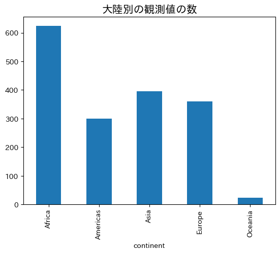
観測値の数#
大陸別の観測値の数
df_group.size()
continent
Africa      624
Americas    300
Asia        396
Europe      360
Oceania      24
dtype: int64
棒グラフ
ax = df_group.size().plot(kind='bar')
ax.set_title('大陸別の観測値の数', size=15)
pass
変数別での観測値の数
df_group.count()
| country | year | lifeExp | pop | gdpPercap | |
|---|---|---|---|---|---|
| continent | |||||
| Africa | 624 | 624 | 624 | 624 | 624 |
| Americas | 300 | 300 | 300 | 300 | 300 |
| Asia | 396 | 396 | 396 | 396 | 396 |
| Europe | 360 | 360 | 360 | 360 | 360 |
| Oceania | 24 | 24 | 24 | 24 | 24 |
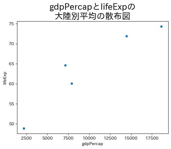
平均#
それぞれの変数の平均(文字列のcountryを含めるとエラーが発生するためthree_varsを指定する。)
df_group[three_vars].mean()
| lifeExp | pop | gdpPercap | |
|---|---|---|---|
| continent | |||
| Africa | 48.865330 | 9.916003e+06 | 2193.754578 |
| Americas | 64.658737 | 2.450479e+07 | 7136.110356 |
| Asia | 60.064903 | 7.703872e+07 | 7902.150428 |
| Europe | 71.903686 | 1.716976e+07 | 14469.475533 |
| Oceania | 74.326208 | 8.874672e+06 | 18621.609223 |
gdpPercapとlifeExpの大陸別平均の散布図
ax = df_group[three_vars].mean().plot(kind='scatter', x='gdpPercap', y='lifeExp')
ax.set_title('gdpPercapとlifeExpの\n大陸別平均の散布図', size=20)
pass
標準偏差#
それぞれの変数の標準偏差
df_group[three_vars].std()
| lifeExp | pop | gdpPercap | |
|---|---|---|---|
| continent | |||
| Africa | 9.150210 | 1.549092e+07 | 2827.929863 |
| Americas | 9.345088 | 5.097943e+07 | 6396.764112 |
| Asia | 11.864532 | 2.068852e+08 | 14045.373112 |
| Europe | 5.433178 | 2.051944e+07 | 9355.213498 |
| Oceania | 3.795611 | 6.506342e+06 | 6358.983321 |
最大値#
df_group.max()
| country | year | lifeExp | pop | gdpPercap | |
|---|---|---|---|---|---|
| continent | |||||
| Africa | Zimbabwe | 2007 | 76.442 | 135031164 | 21951.21176 |
| Americas | Venezuela | 2007 | 80.653 | 301139947 | 42951.65309 |
| Asia | Yemen, Rep. | 2007 | 82.603 | 1318683096 | 113523.13290 |
| Europe | United Kingdom | 2007 | 81.757 | 82400996 | 49357.19017 |
| Oceania | New Zealand | 2007 | 81.235 | 20434176 | 34435.36744 |
最小値#
df_group.min()
| country | year | lifeExp | pop | gdpPercap | |
|---|---|---|---|---|---|
| continent | |||||
| Africa | Algeria | 1952 | 23.599 | 60011 | 241.165876 |
| Americas | Argentina | 1952 | 37.579 | 662850 | 1201.637154 |
| Asia | Afghanistan | 1952 | 28.801 | 120447 | 331.000000 |
| Europe | Albania | 1952 | 43.585 | 147962 | 973.533195 |
| Oceania | Australia | 1952 | 69.120 | 1994794 | 10039.595640 |
3変数の記述統計#
df_group[three_vars].describe().map("{0:.1f}".format).T
| continent | Africa | Americas | Asia | Europe | Oceania | |
|---|---|---|---|---|---|---|
| lifeExp | count | 624.0 | 300.0 | 396.0 | 360.0 | 24.0 |
| mean | 48.9 | 64.7 | 60.1 | 71.9 | 74.3 | |
| std | 9.2 | 9.3 | 11.9 | 5.4 | 3.8 | |
| min | 23.6 | 37.6 | 28.8 | 43.6 | 69.1 | |
| 25% | 42.4 | 58.4 | 51.4 | 69.6 | 71.2 | |
| 50% | 47.8 | 67.0 | 61.8 | 72.2 | 73.7 | |
| 75% | 54.4 | 71.7 | 69.5 | 75.5 | 77.6 | |
| max | 76.4 | 80.7 | 82.6 | 81.8 | 81.2 | |
| pop | count | 624.0 | 300.0 | 396.0 | 360.0 | 24.0 |
| mean | 9916003.1 | 24504795.0 | 77038722.0 | 17169764.7 | 8874672.3 | |
| std | 15490923.3 | 50979430.2 | 206885204.6 | 20519437.6 | 6506342.5 | |
| min | 60011.0 | 662850.0 | 120447.0 | 147962.0 | 1994794.0 | |
| 25% | 1342075.0 | 2962358.8 | 3844393.0 | 4331500.0 | 3199212.5 | |
| 50% | 4579311.0 | 6227510.0 | 14530830.5 | 8551125.0 | 6403491.5 | |
| 75% | 10801489.8 | 18340309.0 | 46300348.0 | 21802867.0 | 14351625.0 | |
| max | 135031164.0 | 301139947.0 | 1318683096.0 | 82400996.0 | 20434176.0 | |
| gdpPercap | count | 624.0 | 300.0 | 396.0 | 360.0 | 24.0 |
| mean | 2193.8 | 7136.1 | 7902.2 | 14469.5 | 18621.6 | |
| std | 2827.9 | 6396.8 | 14045.4 | 9355.2 | 6359.0 | |
| min | 241.2 | 1201.6 | 331.0 | 973.5 | 10039.6 | |
| 25% | 761.2 | 3427.8 | 1057.0 | 7213.1 | 14141.9 | |
| 50% | 1192.1 | 5465.5 | 2646.8 | 12081.7 | 17983.3 | |
| 75% | 2377.4 | 7830.2 | 8549.3 | 20461.4 | 22214.1 | |
| max | 21951.2 | 42951.7 | 113523.1 | 49357.2 | 34435.4 |
groupby.agg()#
agg()を使うと複数のメソッドを同時に使うことができる。この場合は,メソッド名を文字列として引数として使う。
df_group[three_vars].agg("mean")
| lifeExp | pop | gdpPercap | |
|---|---|---|---|
| continent | |||
| Africa | 48.865330 | 9.916003e+06 | 2193.754578 |
| Americas | 64.658737 | 2.450479e+07 | 7136.110356 |
| Asia | 60.064903 | 7.703872e+07 | 7902.150428 |
| Europe | 71.903686 | 1.716976e+07 | 14469.475533 |
| Oceania | 74.326208 | 8.874672e+06 | 18621.609223 |
df_group[three_vars].agg(["max", "min", "mean"])
| lifeExp | pop | gdpPercap | |||||||
|---|---|---|---|---|---|---|---|---|---|
| max | min | mean | max | min | mean | max | min | mean | |
| continent | |||||||||
| Africa | 76.442 | 23.599 | 48.865330 | 135031164 | 60011 | 9.916003e+06 | 21951.21176 | 241.165876 | 2193.754578 |
| Americas | 80.653 | 37.579 | 64.658737 | 301139947 | 662850 | 2.450479e+07 | 42951.65309 | 1201.637154 | 7136.110356 |
| Asia | 82.603 | 28.801 | 60.064903 | 1318683096 | 120447 | 7.703872e+07 | 113523.13290 | 331.000000 | 7902.150428 |
| Europe | 81.757 | 43.585 | 71.903686 | 82400996 | 147962 | 1.716976e+07 | 49357.19017 | 973.533195 | 14469.475533 |
| Oceania | 81.235 | 69.120 | 74.326208 | 20434176 | 1994794 | 8.874672e+06 | 34435.36744 | 10039.595640 | 18621.609223 |
自作の関数も使用することができる。この場合は,関数名だけを使う(文字列ではない)。
func = lambda x: ( np.max(x)-np.min(x) )/np.mean(x)

df_group[['lifeExp','pop','gdpPercap']].agg(func)
| lifeExp | pop | gdpPercap | |
|---|---|---|---|
| continent | |||
| Africa | 1.081401 | 13.611447 | 9.896297 |
| Americas | 0.666174 | 12.261971 | 5.850528 |
| Asia | 0.895731 | 17.115583 | 14.324219 |
| Europe | 0.530877 | 4.790574 | 3.343843 |
| Oceania | 0.162998 | 2.077754 | 1.310079 |
continentの内訳の割合を計算
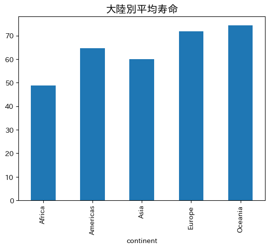
図#
continent平均寿命
df_lifeExp_continent = df_group['lifeExp'].mean()
ax = df_lifeExp_continent.plot(kind='bar')
ax.set_title('大陸別平均寿命', size=15)
pass
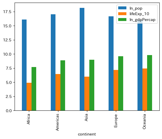
3つの変数#
df_mean = df_group[three_vars].mean()
df_mean['ln_pop'] = np.log( df_mean['pop'] )
df_mean['ln_gdpPercap'] = df_mean['gdpPercap'].apply(np.log)
df_mean['lifeExp_10'] = df_mean['lifeExp']/10
df_mean[['ln_pop','lifeExp_10', 'ln_gdpPercap']].plot(kind='bar')
pass
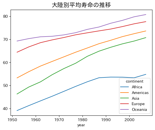
複数階層のgroupby()#
continent別の平均時系列を考えるときに有用。
df_group2 = df.groupby(['continent','year'])
df_group2[three_vars].mean().head()
| lifeExp | pop | gdpPercap | ||
|---|---|---|---|---|
| continent | year | |||
| Africa | 1952 | 39.135500 | 4.570010e+06 | 1252.572466 |
| 1957 | 41.266346 | 5.093033e+06 | 1385.236062 | |
| 1962 | 43.319442 | 5.702247e+06 | 1598.078825 | |
| 1967 | 45.334538 | 6.447875e+06 | 2050.363801 | |
| 1972 | 47.450942 | 7.305376e+06 | 2339.615674 |
lifeExpの列だけを選択した後,.unstack()を使ってyearが行ラベルになるDataFrameに変換してみる。
df_lifeExp_group = df_group2[three_vars].mean().loc[:,'lifeExp'].unstack(level=0)
ax = df_lifeExp_group.plot()
ax.set_title('大陸別平均寿命の推移', size=15)
pass
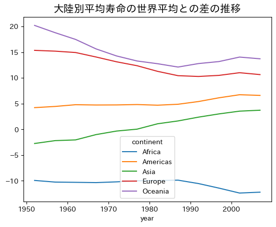
世界平均との比較
df_group_year = df.groupby('year')
world_lifeExp = df_group_year[three_vars].mean()['lifeExp'].to_numpy().reshape(1,12).T
df_lifeExp_diff = df_lifeExp_group - world_lifeExp

ax = df_lifeExp_diff.plot()
ax.set_title('大陸別平均寿命の世界平均との差の推移', size=15)
pass